Introduction

This is a demo script for Image Histogram Equalization. This type of image transformation is useful as a global/local contrast enhancer; however, if not being used correctly, generally generates an irrealistic color image.

Matlab already provides an implementation of this pointwise operation (imhist), however for testing purpose I would like to study the implementation in different languages. I will post in the following days version for different languages/library (my target are CUDA, openCL and openGL).

Note: think this article as a scratch-pad, I will update this as a reference example of image processing in different programming languages.

Steps of the algorithm:

1. The input RGB image is converted into grayscale image. Alternatively, we can calculate the equalized image for each channel independently. I will follow the grayscale image. FH(r). Pixel amplitude is in the [0..255] interval, the usual uint8 type;
2. Calculate the probability of each value: for a N*M image, the probability is Pr(r)=FH(r)/(N*M);
3. Find the Cumulative Distribution, CD(r)
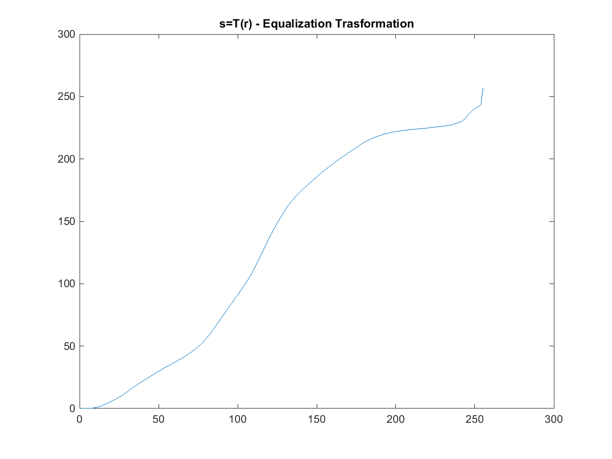
4. The s=T(r) function is Lmin+CD(r)*(Lmax-1), where [Lmin..Lmax] is the range we want in the final image
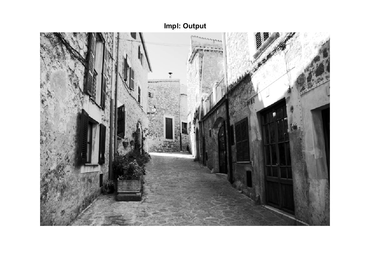
5. Apply the transformation: Input image: f(x,y); the output image f'(x,y)=T(f(x,y))

I will start with a manual implementation in matlab, as a reference implementation.

Matlab implementation

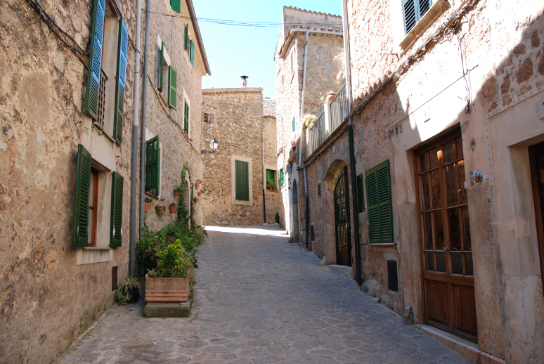
Original image (RGB and grayscale version):

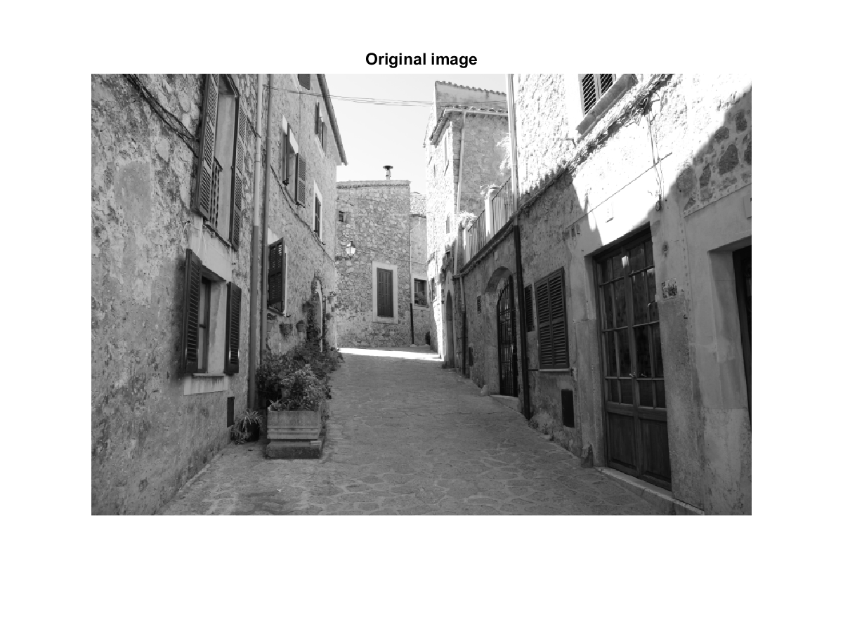
 I convert this image in the corresponding Luminance (grayscale) version:

 

 

 

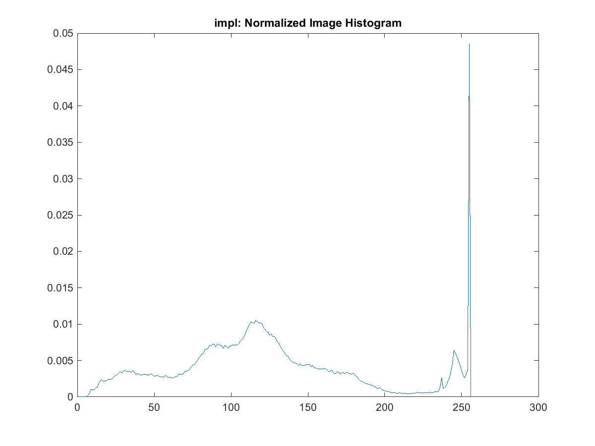
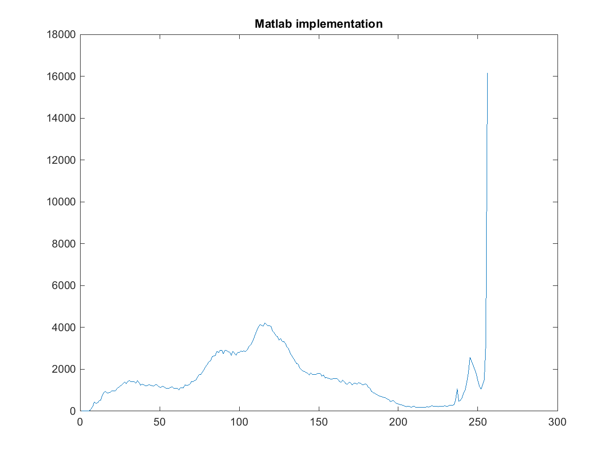
From the grayscale version, the first step is to generate the histogram of uint8 values; I generate the histogram manually, then using the imhist() matlab function:

Then I apply the Histogram Equalization, after calculating the pointwise s=T(r) mapping function:

The result of applying the T(r) function to the original grayscale image:

 

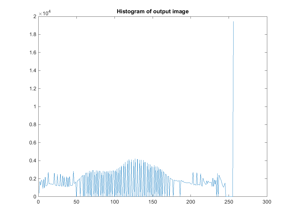
with this Histogram:

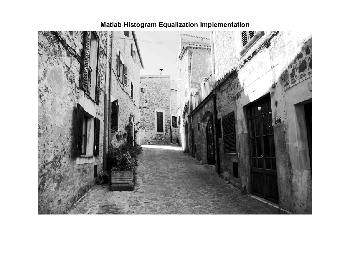
The corrisponding matlab version is the following:

How the two version differentiate?

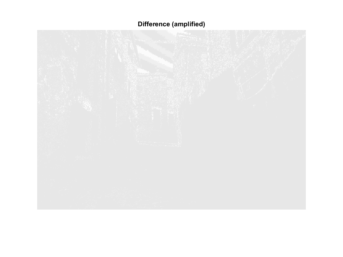
the statistical difference between the two output grayscale images:

Min value = 0  Max value = 3  mean=0.151163  std_dev=0.486329

 

Matlab source code

This is the Matlab source code used in this implementation. There are many other possible implementations around, but I would like to explicit many transformations generally done using very few Matlab built-in functions.

 

%% Equalizzazione - ex1.m
EXDIR = '..\images\';
FN = strcat(EXDIR, 'input_0.png');

I = imread(FN);
GS = rgb2gray(I);

GSV = GS(:);
freq = uint32(zeros(256, 1));
s = length(GSV);
disp (sprintf ('Min value = %f  Max value = %f', min(GSV), max(GSV)));
for i = 1:s
    freq(GSV(i) + 1) = freq(GSV(i) + 1) + 1;
end
n_freq = double(freq) / s;
P = figure;
plot (n_freq);
title ('impl: Normalized Image Histogram');
saveas (P, 'output\man_histogram.png');
%%
P = figure;
MI = imhist(GS);
plot (MI);
title ('Matlab implementation');
saveas (P, 'output\mat_histogram.png');

%% Apply Histogram Equalization Function
P = figure;
imshow(GS);
title ('Original image');
saveas (P, 'output\gs_input.png');

% Histogram with Pr(r) values (normalized frequency)

Pr = n_freq;
L = 256;
T = zeros(256, 1);
T(1) = n_freq(1);
for i = 2:256
    T(i) = T(i - 1) + Pr(i);
end
T = T * L;
P = figure;
plot(T);
title ('s=T(r) - Equalization Trasformation');
saveas (P, 'output\man_pointwise_function.png');

%% Execute
GS2 = uint8(zeros(s, 1));
for i = 1:s
    GS2(i) = T(GSV(i) + 1);
end

Out = reshape (GS2, size(GS));
P = figure;
imshow(Out);
title ('Impl: Output');
saveas(P, 'output\man_output.png');

P = figure;
plot(imhist(Out));
title ('Histogram of output image');
saveas (P, 'output\man_output_hist.png');

%% Matlab implementation
V = histeq(GS);
P = figure;
imshow(V);
title ('Matlab Histogram Equalization Implementation');
saveas (P, 'output\mat_pointwise_function.png');

%% Comparison
Diff = abs(V - Out);
P = figure;
disp (sprintf ('Difference:Min value = %d  Max value = %d  mean=%f  std_dev=%f', min(Diff(:)), max(Diff(:)), mean(Diff(:)), std(double(Diff(:)))));
imshow(histeq(Diff));
title ('Difference (amplified)');
saveas (P, 'output\diff.png');